Simulating in local/world space

ObiSolver can perform the simulation in one of two spaces: world space (the default) and local space. Here we will describe how to set up both, and the differences between them.

World space

When simulating in world space, all simulation data (particle positions, velocities, accelerations, etc) will be expressed using the world as a reference frame.

No special setup is required to work in world space. Both the solver and the actors can be anywhere in the scene.

Advantages:

• No special setup needed, easy to use.
• The solver and any actors simulated by it can be anywhere in the scene hierarchy.

Disadvantages:

• If an actor is very far away from the world's origin, floating point precision will degrade. This will result in choppy/unstable simulation, and can become a problem in very large game worlds.
• You have no control over inertial forces. This can make it difficult to fine tune certain effects such as character clothing.
• If multiple prefab actors are meant to share a single solver in the scene, you will have to manually re-add the actor instances to the solver at runtime.

Local space

When simulating in local space, all simulation data (particle positions, velocities, accelerations, etc) will be expressed using the solver's transform as the reference frame.

Advantages:

• Offers fine control over inertial forces, both linear and angular. This is very useful under some circumstances, such as character clothing.
• The simulation can be very far away from the world's origin and still retain excellent floating point precision, as all quantities are expressed with respect to the solver's transform.
• Allows to translate/rotate/scale the entire simulation result by scaling the solver transform.

Disadvantages:

• It requires deeper understanding of vector spaces and inertial forces, and needs to be correctly set up.
• There's a slight performance overhead associated with simulating in local space.

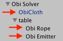
To set up local space simulation, enable "Simulate in local space" in the ObiSolver inspector. Then, make sure all actors that are being simulated by that solver are below it in the hierarchy.

When local space simulation is enabled in the solver, 4 new parameters will appear under it:

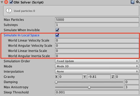
World linear velocity scale

Controls how much of the world-space linear velocity of the solver transform is applied to the particles. Typical values range from 0 (none) to 1 (all of it), though values outside of this range can be used for non-physical effects.

World angular velocity scale

Analogous to the previous property, but controls angular velocity (rotations) instead of linear velocity (translations).

World linear inertia scale

Controls how much of the world-space linear inertia of the solver transform is applied to the particles. Typical values range from 0 (none) to 1 (all of it), though other values can be used for non-physical effects.

World angular inertia scale

Analogous to the previous property, but controls angular inertia (rotations) instead of linear inertia (translations). Note that centrifugal and coriolis forces are accounted for.

A quick reminder about the difference between velocity and inertia: inertia is the resistance to a change in velocity. Imagine for a moment that you drive a car with a pair of plush dice hanging from the rearview mirror. While the car is moving at a constant speed, the dice are hanging perfectly still. No velocity from the car is being "transferred" to the dice (world linear velocity scale = 0). If you suddenly hit the brakes, the car would abruptly stop and the dice would swing forward. Here, inertia is trying to keep the dice moving at the same speed they were before the car stopped (world linear inertia scale = 1). You can clearly see this effect in the gif for linear inertia scale: